Shapely 扩展包功能札记 |
您所在的位置:网站首页 › Linestring python › Shapely 扩展包功能札记 |
Shapely 扩展包功能札记
|
Shapely 扩展包功能札记
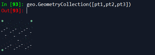
shapely 是python 中开源的空间几何对象库,支持 Point(点),LineString(线),Polygon(面) 等几何对象及相关空间操作。 Shapely is a BSD-licensed Python package for manipulation and analysis of planar geometric objects. It is based on the widely deployed GEOS (the engine of PostGIS) and JTS (from which GEOS is ported) libraries. Shapely is not concerned with data formats or coordinate systems, but can be readily integrated with packages that are 目录 Shapely 扩展包功能札记 参考网址 安装 下面会列出代码的 Shapely 功能 代码展示 1. 几何对象和 numpy.array 之间互相转换 2. 求解线的长度,面的面积,对象之间的距离,最小最大距离 3. 几何对象之间的关系判定:相交 (intersect),包含 (contain),相交区域 (intersection) 4. 对几何对象求几何中心 (centroid),缓冲区 (buffer),最小旋转外界矩形 (minimum_rotated_rectangle) 5. 求线的插值点 (interpolate),求点投影到线的距离 (project),求几何对象之间对应的最近点 (nearestPoint) 6. 对几何对象进行旋转 (rotate) 和缩放 (scale)。 总结 参考网址 官方资料:Shapely documentation30 分钟学会 shapely 空间几何分析Datawhale 组队学习资料 安装本人一开始需要安装的是 GDAL 包,但是因为 Shapely 包版本不对所以将其卸了重装,因为要下载与GDAL相对应的版本,所以是通过 whl 文件安装 Shapely ,主要参考了知乎一位博主的博文 《geopandas安装心得(win10)》。如果只需要安装 shapely 包,不需要考虑版本的问题,那直接 利用 Anaconda Prompt 通过命令: $ pip install shapely就可以安装。如果需要安装特定版本的 Shapely 包,那可以和我一样通过 whl 文件进行安装,具体的安装流程可以参考上面的知乎链接。(不使用 conda 安装的原因主要是网络问题,一直装不上,网好的同学可以考虑用 conda 安装一劳永逸) 提示:以下是本篇文章正文内容,所有案例都是通过 Spyder (python 3) 进行演示。来看这篇博文的相信都是某几个命令搞不清楚的,那就直接干货! 下面会列出代码的 Shapely 功能 几何对象(点、线、面)和numpy.array互相转换;求解线的长度,面的面积,对象之间的距离,最小最大距离;几何对象之间的关系判定:相交 (intersect),包含 (contain),相交区域 (intersection) ;对几何对象求几何中心 (centroid),缓冲区 (buffer),最小旋转外界矩形 (minimum_rotated_rectangle) 等;求线的插值点 (interpolate),求点投影到线的距离 (project),求几何对象之间对应的最近点 (nearestPoint);对几何对象进行旋转 (rotate) 和缩放 (scale)。下面对上述六种命令进行一一展示。 代码展示 1. 几何对象和 numpy.array 之间互相转换导入必要的包: from shapely import geometry as geo from shapely import wkt from shapely import ops import numpy as np创建点、线、面对象,其中三种对象各自的第二种创建方法 #2 都是利用 numpy 数组的方法进行创建: ## TODU: 创建点 Point 对象(三种方法) pt1 = geo.Point([0,0]) # 1 coord = np.array([0,1]) pt2 = geo.Point(coord) # 2 pt3 = wkt.loads("POINT(1 1)") # 3 ## TODU: 创建线 LineString 对象 (三种方法) line1 = geo.LineString([(0,0),(1,-0.1),(2,0.1),(3,-0.1),(5,0.1),(7,0)]) # 1 arr = np.array([(2,2),(3,2),(4,3)]) line2 = geo.LineString(arr) # 2 line3 = wkt.loads("LineString(-2 -2,4 4)") # 3 ## TODU: 创建面 Polygon 对象 (四种方法) poly1 = geo.Polygon([(0,0),(1,0),(1,1),(0,1),(0,0)]) #起点和终点相同 # 1 coords = np.array([(0,0),(1,0.1),(2,0),(1,2),(0,0)]) poly2 = geo.Polygon(coords) # 2 poly3 = wkt.loads("POLYGON((0 0,2 0,2 2,0 2,0 0),(0.5 0.5,1.5 0.5,1.5 1.5,0.5 1.5,0.5 0.5))") # 3 poly4 = geo.Polygon.from_bounds(xmin=0,ymin=0,xmax=20,ymax=20) # 4对象可视化,对应上面三种对象的创建方式里的变量命名。 # 点对象 批量可视化 geo.GeometryCollection([pt1,pt2,pt3]) # 线对象 可视化 geo.GeometryCollection([line2]) # 面对象 可视化 geo.GeometryCollection([poly3])对应三种对象可视化的 Spyder 运行结果如下图所示: 点对象 批量可视化:
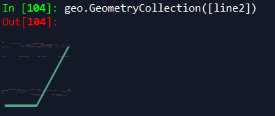
线对象 可视化:
面对象 可视化:
2. 求解线的长度,面的面积,对象之间的距离,最小最大距离 点对象、线对象、面对象之间的距离: ## 点对象:点 pt2 与点 pt1 之间的距离 d (线段 pt1 -> pt1 的长度) d = pt2.distance(pt1) # 点点距离 ## 线对象:线 line1 与线 line2 之间的距离 d1 = line1.distance(line2) # 线线距离 d2 = line1.distance(geo.Point([-1, 0])) # 线点距离 d3 = line1.hausdorff_distance(line2) # 最大最小距离(线段之间) ## 面对象:面积与周长 s1 = poly1.area # 面对象面积 c1 = poly1.length # 面对象周长 exte = np.array(poly1.exterior) # 面对象外围坐标点 bds = poly3.bounds # 面对象坐标范围3. 几何对象之间的关系判定:相交 (intersect),包含 (contain),相交区域 (intersection) 点、线、面对象关系判定: # 线线关系 jug1 = line2.intersects(line3) # 线线是否相交 True or False intpt1 = line2.intersection(line3) # 线线交点坐标 (可以通过 np.array() 显示坐标值) # 点线关系 jug2 = line2.contains(geo.Point(2.5,2)) # 线(段)是否包含点 True or False # 面点关系 jug3 = poly2.contains(geo.Point(0,0)) # 面是否包含点 True or False # 面线关系 jug4 = poly2.intersects(geo.LineString([(0,0),(5,5)])) # 面线是否相交 True or False inte1 = poly1.intersection(line3) # 面线交集 # 面面关系 jug5 = poly2.intersects(poly3) # 面面是否相交 True or False inte2 = poly1.intersection(poly2) # 面面交集 uni1 = poly1.union(poly2) # 面面并集 diff1 = poly2.difference(poly1) # 面面补集4. 对几何对象求几何中心 (centroid),缓冲区 (buffer),最小旋转外界矩形 (minimum_rotated_rectangle) 线、面对象几何中心确定: # 线几何中心 center = line2.centroid geo.GeometryCollection([line2,center]) # 线段及其几何中心显示 # 面几何中心 center = poly3.centroid geo.GeometryCollection([center,poly3]) # 面及其几何中心显示点、线、面缓冲区确定: # 点、线、面缓冲区扩展都是一样的格式:obj.buffer(distance, cap_style = 1/2/3, join_style = 1/2) # 点对象缓冲区 buffer_pt1 = pt1.buffer(0.1) # 点按圆形扩展缓冲区 geo.GeometryCollection([pt1, buffer_pt1]) # 线对象缓冲区 buffer_line2_11 = line2.buffer(0.2, cap_style = 1, join_style = 1) # 端点半圆扩展, 圆弧链接 buffer_line2_21 = line2.buffer(0.2, cap_style = 2, join_style = 1) # 端点不扩展, 圆弧链接 buffer_line2_31 = line2.buffer(0.2, cap_style = 3, join_style = 1) # 端点方形扩展, 圆弧链接 buffer_line2_12 = line2.buffer(0.2, cap_style = 1, join_style = 2) # 端点半圆扩展, 折角链接 # 面对象缓冲区 buffer_poly_bigger = poly2.buffer(0.2) # 面对象面积外扩 buffer_poly_smaller = poly2.buffer(-0.2) # 面对象面积内缩 print(buffer_poly_smaller.area) # 计算内缩对象的面积最小外接矩形、最小旋转外接矩阵: # 线对象 enve_line = line2.envelope # 最小外接矩形 rot_rect_l = line2.minimum_rotated_rectangle # 最小旋转外接矩形 # 面对象 enve_poly = poly2.envelope # 最小外接矩形 rot_rect_p = poly2.minimum_rotated_rectangle # 最小旋转外接矩形Spyder 显示:
5. 求线的插值点 (interpolate),求点投影到线的距离 (project),求几何对象之间对应的最近点 (nearestPoint) 求线的插值点: pt_half = line1.interpolate(0.5, normalized = True) geo.GeometryCollection([line1, pt_half])Spyder 显示:
求点投影到线的距离: # 投影 ratio = line1.project(pt_half, normalized=True) print(ratio)求几何对象之间的最近点: # 导入 shapely.ops 包 from shapely import ops poly1 = geo.Polygon([(0,0), (2,0), (1,1), (0,0)]) poly2 = geo.Polygon([(4,0),(6,0),(6,2),(4,2),(4,0)]) # 求取两个面对象相距最近点的坐标 p1, p2 = ops.nearest_points(poly1,poly2) geo.GeometryCollection([poly1,poly2,p1,p2])Spyder 显示:
6. 对几何对象进行旋转 (rotate) 和缩放 (scale)。 旋转、平移、缩放几何对象: # 导入必要的包 from shapely import affinity ## (顺时针)旋转 # shapely.affinity.rotate(geom, angle, origin='center', use_radians=False) line = LineString([(1, 3), (1, 1), (4, 1)]) rotated_a = affinity.rotate(line, 90) rotated_b = affinity.rotate(line, 90, origin='centroid') geo.GeometryCollection([line, rotated_a]) ## 缩放 # shapely.affinity.scale(geom, xfact=1.0, yfact=1.0, zfact=1.0, origin='center') triangle = Polygon([(1, 1), (2, 3), (3, 1)]) triangle_a = affinity.scale(triangle, xfact=1.5, yfact=-1) triangle_a.exterior.coords[:] geo.GeometryCollection([triangle, triangle_a]) triangle_b = affinity.scale(triangle, xfact=2, origin=(1,1)) triangle_b.exterior.coords[:] geo.GeometryCollection([triangle, triangle_b]) ## 平移 # shapely.affinity.translate(geom, xoff=0.0, yoff=0.0, zoff=0.0) triangle = Polygon([(1, 1), (2, 3), (3, 1)]) triangle_a = affinity.translate(triangle, xoff=1.0, yoff=2.0) geo.GeometryCollection([triangle, triangle_a])Spyder 显示: 旋转
总结 以上就是今天要讲的内容,本文仅仅简单介绍了 shapely 部分功能的使用,而 shapely 提供了大量能使我们快速便捷地处理数据的函数和方法,如果需要深入使用 shapely 的功能,看这篇介绍肯定是远远不够的,最好的方式就是看 shapely 的官方介绍文档,相信一定能收获颇多。 |


【本文地址】